When you make a workbook in Google Sheets that contains a lot of worksheet tabs, finding the important ones can be difficult. In some cases you might actually need to access every tab in your worksheet but, in other cases, there might be some old tabs or tabs that are just for formula references, which probably don’t need to be visible. These situations are great options for hidden tabs. A hidden tab in Google Sheets is still actually a part of the file, but it’s hidden from view so that the tab isn’t taking up space, and so that you don’t accidentally edit information on the wrong tab. Our guide below will show you how to hide a worksheet tab in Google Sheets.
How to Hide a Worksheet Tab in Google Sheets
Our guide continues below with more information on hiding worksheet tabs in Google Sheets, including pictures of these steps. Note that once you select Hide sheet from the right-click menu that you will be hiding tabs from anyone that can open the file, not only the people that you don’t want to see them.
How to Create A Hidden tab in Google Sheets (Guide with Pictures)
The steps in this article are going to show you how to hide an existing tab in a Google Sheets file. You will still be able to create formulas that use cells in this hidden worksheet, and you will be able to unhide the worksheet later if you so choose.
Step 1: Sign in to your Google Drive and open the Google Sheets file containing the worksheet tab that you would like to hide.
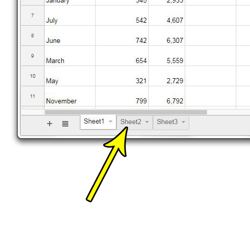
Step 2: Locate the worksheet tabs at the bottom of the window.
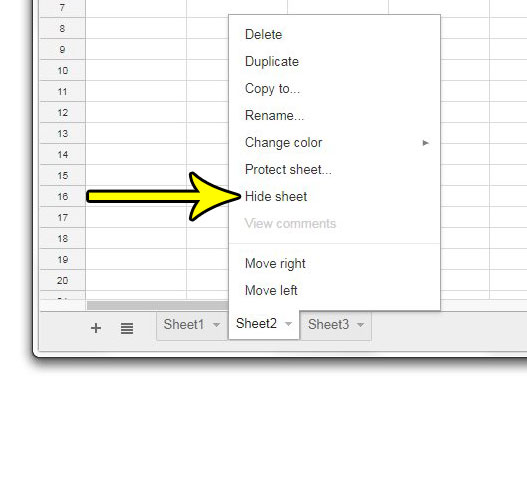
Step 3: Right-click on the worksheet tab that you want to hide, then select the Hide sheet option.
After you click Hide sheet then the selected sheet will no longer be visible at the bottom of the window. You can then continue to hide tabs that you want to hide from other spreadsheet editors or people that are viewing the file. You will also see a little popup that tells you how to find and unhide worksheets later but, in case you would like to see those steps as well, then find out how to unhide in Google Sheets if you find that you need to edit something, or view something, on a sheet that is hidden.
How to Unhide a Worksheet Tab or Hidden Sheets in Google Sheets
If you have a worksheet tab with “finished” data, or if the data on that tab simply isn’t very important, then you may well never need to view or edit it again. But if you have a hidden tab or hidden sheet tabs and you need to unhide it, then you are able to do so. To unhide a tab in Google Sheets you can click the View tab at the top of the window, select Hidden sheets, then click the worksheet that you want to unhide. You can also unhide a worksheet tab in Google Sheets by clicking the three horizontal lines at the bottom-left of the window, then click on the worksheet that you want to unhide. Note that you aren’t able to unhide two or more sheets at the same time.
How to Hide Multiple Worksheet Tabs in Google Sheets
If you have a lot of worksheet tabs that you want to hide then you can speed this process up a little bit. If you hold down the Ctrl key on your keyboard you can click on each worksheet tab that you want to hide. If you want to hide a range of adjacent worksheet tabs then you can click the leftmost sheet tab, hold down the Shift key, then click the rightmost sheet tab to select all of the worksheets between them as well. You can then right-click a selected tab and choose the Hide sheets option. Once all of the tabs are selected, simply right-click on one of those tabs and choose the Hide sheets option. Unfortunately, there isn’t a way to unhide multiple worksheet tabs in Google Sheets. You will need to unhide them manually, or download the file in the Microsoft Excel format, open it in Excel, and unhide them all that way. You can download a Google Sheets file in the Excel format by clicking File at the top of the window, choosing Download, then selecting the Microsoft Excel option. This will create a copy of your Google Sheets file in the Excel format and download it to your computer. You can unhide all of your worksheet tabs in Microsoft Excel by right-clicking on a worksheet tab and choosing the Unhide option, then clicking the top sheet, holding down the Shift key, then clicking the bottom sheet. Once all of the hidden worksheets are selected you can click the OK button.
More Information on How to Use the Google Sheets Hide Sheet Tab Setting
Hiding worksheets in Google Apps or Microsoft Office spreadsheet editors is a quick and usually effective way to protect your data entry from people with the same permissions for the file as you. It can help to limit editing by making the data tougher to find, as people will need to take several extra steps to view the certain cells or sheets that you elected to hide. I often use the hide sheet option in Google Sheets when I have a sheet in my workbook that contains a lot of important data for my formulas, and I don’t want someone to accidentally delete or edit the data that is on that sheet. Another option that you could employ involves locking the worksheet or the cells containing your important data. This is a little tougher, but it is a more effective solution if you think that someone else with access to your spreadsheet could edit the data that you don’t want them to edit. You can accomplish this by protecting a range of cells or a sheet. To do this select the Data tab at the top of the window, then choose the Protect sheet and ranges option. You can then click the Add a sheet or range option in the Protected sheets & ranges column at the right side of the window, then choose the range of cells or the worksheet that you want to protect. You then click the Set permissions button and choose what you would like to happen. You can either show a warning or format the selection so that only you can edit it.
Additional Reading
He specializes in writing content about iPhones, Android devices, Microsoft Office, and many other popular applications and devices. Read his full bio here.


