One way that you can fix this problem, if your data is currently in a row and you need it to be in a column instead, is to paste that horizontal data into a vertical layout. This is accomplished with a Paste option called Transpose, and it can really be a time saver. So continue reading our article below to see how you can paste from horizontal to vertical in Excel 2013.
How to Copy a Row of Cells and Paste Them Into a Column in Excel 2013
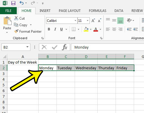
The steps in this article were performed in Microsoft Excel 2013. However, these will also work in Excel 2010 and Excel 2016. Note that this will work best if you are pasting into empty cells. Otherwise you may lose the data in the cells where you are pasting your copied data. Step 1: Open your spreadsheet in Excel 2013. Step 2: Select the horizontal cells that you would like to paste vertically.
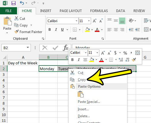
Step 3: Right-click the selected cells, then choose the Copy option. Note that you can also press Ctrl + C on your keyboard to copy instead.
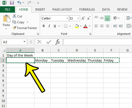
Step 4: Click in the cell where you wish to display the first vertical cell.
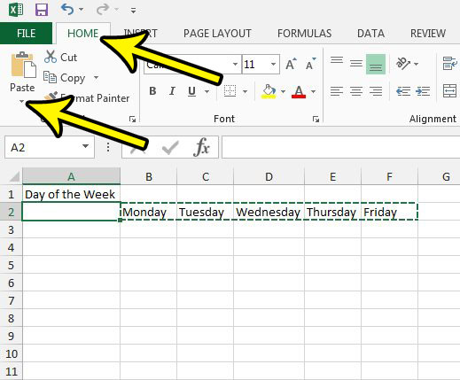
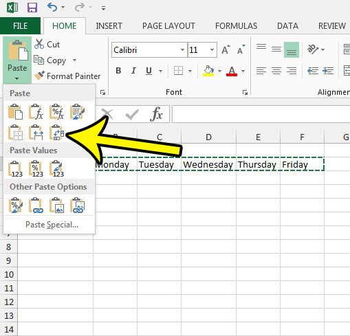
Step 5: Click the Home tab at the top of the window, then click the small arrow under the word Paste.
Step 6: Click the Transpose option on the Paste dropdown menu.
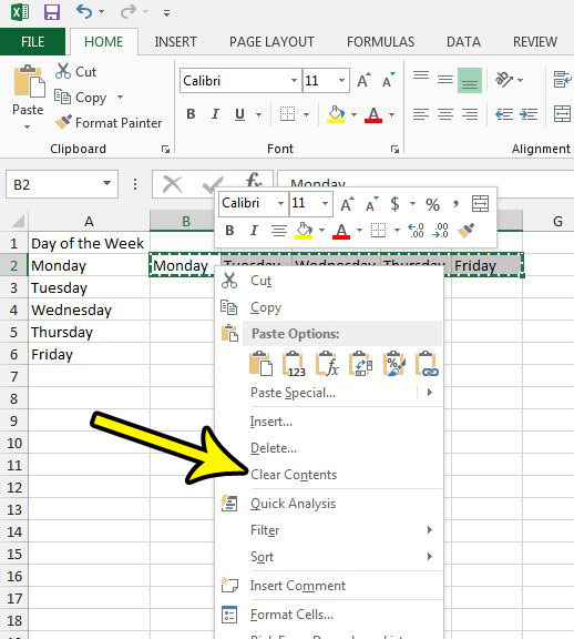
Step 7: If the cells are now displaying how you would like them to, you can right-click the original horizontal data, then click the Clear Contents option to delete it without affecting the layout of the rest of the spreadsheet.
Are you having trouble getting your spreadsheet to print properly? Read our guide on Excel print optimization for some tips and tricks that can help you to solve the frustration that you might be experiencing. He specializes in writing content about iPhones, Android devices, Microsoft Office, and many other popular applications and devices. Read his full bio here.
