A spreadsheet with a lot of data can easily become unruly. While you may have previously experimented with hiding and unhiding rows and columns, but that can be tedious when you need to constantly change the viewability of rows or columns. Luckily there is an option in Microsoft Excel that lets you group a set of rows. This adds an extra section of controls to the left of the spreadsheet that you can use to quickly hide or show a selection of rows. Our guide below is going to show you how to group rows in Excel for Office 365 so that you can take advantage of these options.
How to Create a Group of Rows in Microsoft Excel for Office 365
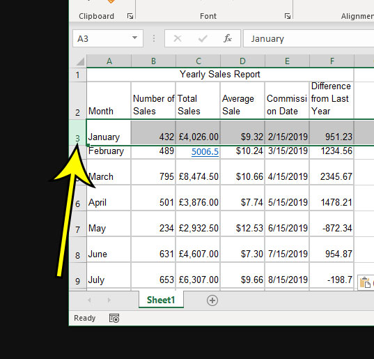
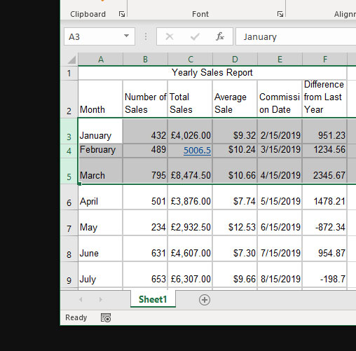
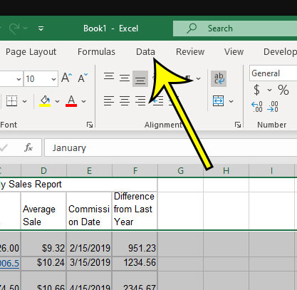
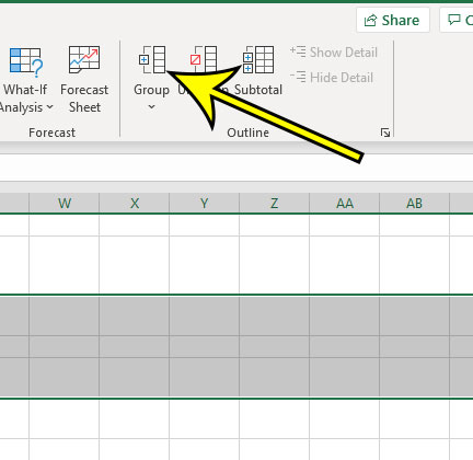
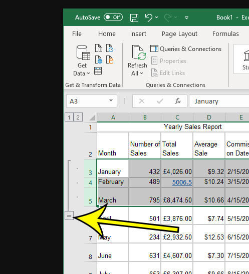
The steps in this article were performed in the Excel for Office 365 version of the application but will also work in other versions of Excel such as Excel 2013, Excel 2016, or Excel 2019. Step 1: Open the Excel file containing the rows that you want to group. Step 2: Click on the first row number that you want to include in the group. Step 3: Hold down the Shift key on your keyboard and click the bottom row number to include in the group. Step 4: Select the Data tab at the top of the window. Step 5: Click the Group button in the Outline section of the ribbon. You should now see a new section of options to the left of your row numbers. You can click the minus button to hide this group. You can then click the plus button to unhide it. Find out how to freeze a row in Microsoft Excel if you would like to keep that row visible at the top of the spreadsheet as you scroll down. He specializes in writing content about iPhones, Android devices, Microsoft Office, and many other popular applications and devices. Read his full bio here.